II-1 Changing Parameters from the GUI

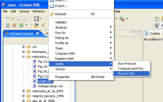
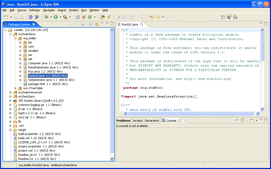
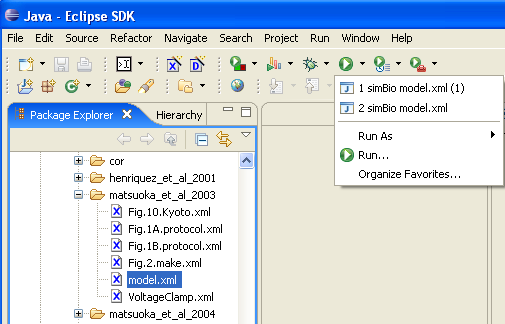
To run the model, in the Eclipse Package Explorer view, in the simBio project select src/xml/matsuoka_et_al_2003/model.xml, and right click. Then, click on [simBio]->[Run on GUI] in the popup menu.

set up by hand

Select org.simBio.RunGUI.java.

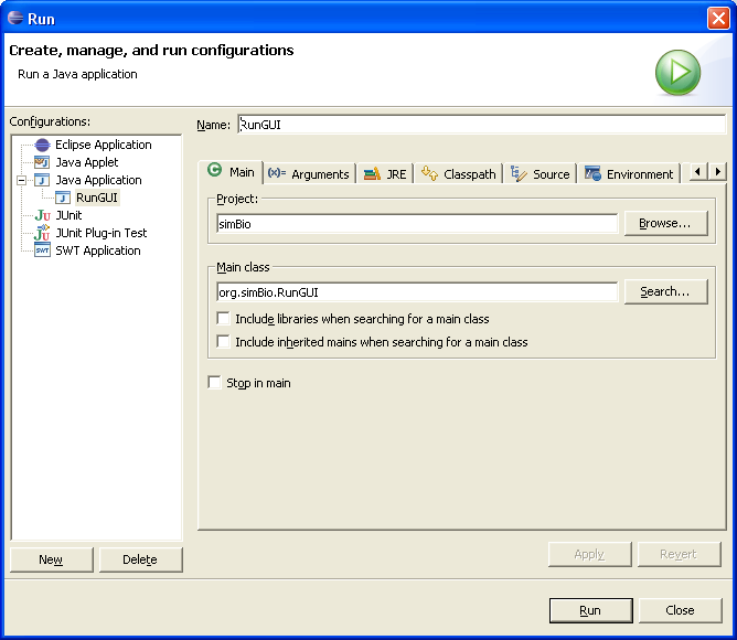
In the menu select "Run" -> "Run...". Please push the "New" button under the left.

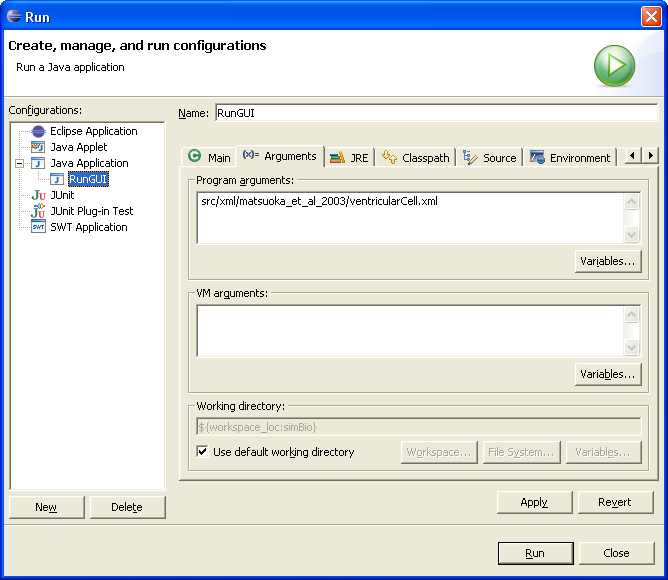
Input the model XML file name which you would like to execute in the box "Program arguments" of the "Arguments" tab. Example "src/xml/matsuoka_et_al_2003/model.xml". Click "Run".

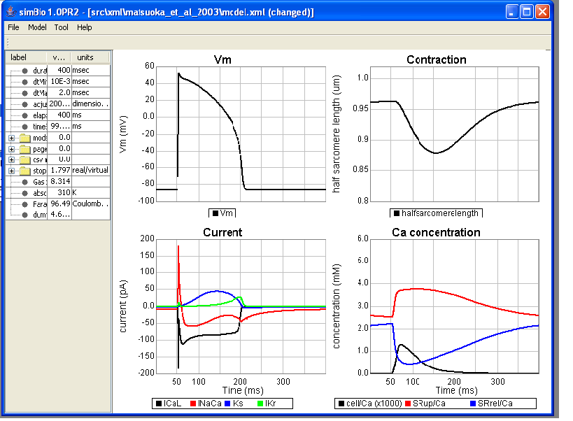
The simBio GUI starts, and the model is read in. When you click on [Model]->[Start] in the menu, the matsuoka_et_al_2003 model runs on simBio, and curves are drawn like in the Figure below.

starting structure

When you run it one time the starting structure is saved, so from the second time onwards you can run it from the coolbar.

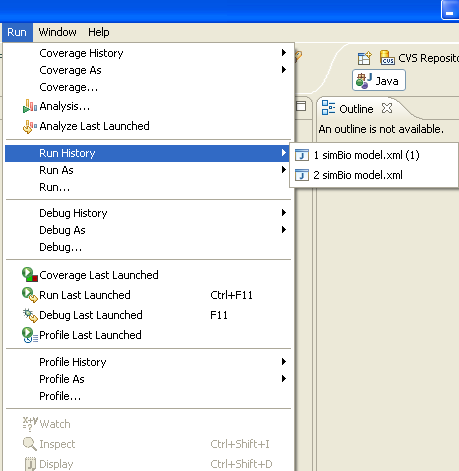
Alternatively, you can start it in the menu from [Run]->[Run Last Launched] or select one from [Run History].

It's convenient to do this

In the initial state, the tool bar is a blank space. Please edit it in [Tool]->[Option]. For details, please refer to [Help]->[GUI]->[Menu]->[Tool]->[Option ... Show toolbar maintainance dialog].

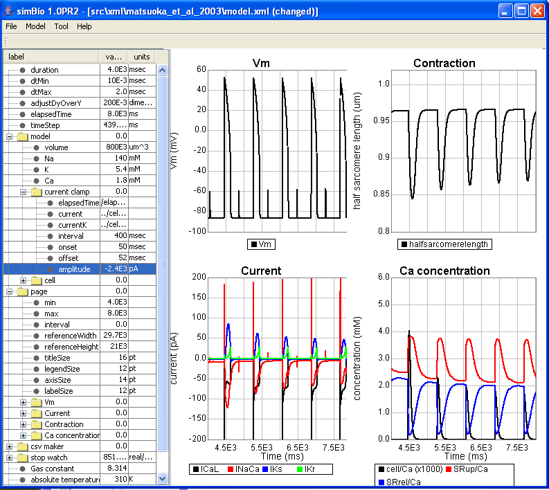
On the left, the parameter tree table is displayed, on the right, a graph showing heart muscle cell activity.

The horizontal axis of the graph is time (ms), and the top left graph shows action potential, in the bottom left L-type Ca current (ICaL), Na/Ca exchange current (INaCa), fast component (IKs) and slow component (IKr) of delayed rectifier K current, cytoplasm Ca concentration in the lower right (cell/Ca), Ca concentration of the sarcoplasmic reticulum Ca uptake region (SRup/Ca), Ca concentration of the Ca release region (SRrel/Ca), half sarcomere length in the top right (halfsarcomerelength).

The heart performs the task of pumping blood through the entire body. In other words, it can be said that the function of ventricular myocytes is contraction. Beginning from the pacemaker cells, the action potential expands into the entire heart and brings about a contraction.

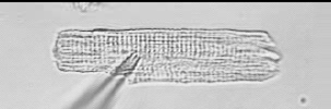
The heart consists of muscle cells like in Figure 2-1-6. In the Figure, the cell is excited by a stimulus from a glass electrode stretching from the bottom left, and contracts.

When a cardiac muscle cell contracts, the elements shown in Figure 2-1-7 interact.

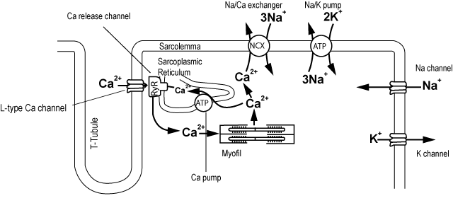
The resting cell membrane potential is kept at -90 mV, because of the ion concentration gradient inside and outside the cell. This state is described as polarization. When the electrical potential inside a cell becomes shallow, this is called depolarization, and when a depolarized potential returns to its previous potential, this is called repolarization.

There are channels which passively allow ions to pass through the cell membrane, and there are pumps and transporters which actively transport them using energy, selectively transporting the ions. The movement of ions which have electrical charge also generates current and exerts an influence on membrane potential and ion concentration. Furthermore, the channels have a gate structure, which depends on the electric potential and ion concentration, and changes the permeability of ions.

The action potential is the change in potential when the membrane potential transiently depolarizes and repolarizes due to the passage of ions through the cell membrane. The shape is different according to the type of cell. In the matsuoka_et_al_2003 model, when an electrical stimulus is applied at time 50 ms, Na⁺ channels open and the membrane depolarizes. Then K⁺ channels open and the membrane repolarizes, which forms an action potential.

When a cell membrane depolarizes, L-type Ca²⁺ channels on the T-tubule open and there is an influx of Ca²⁺ into the cell. Ca²⁺ which has entered from L-type Ca²⁺ channels open Ryanodine channels in the vicinity that release Ca²⁺ from sarcoplasmic reticulum. Then, the concentration of Ca²⁺ in cytoplasm ([Ca²⁺]_i) rises at once. The released Ca²⁺ acts on troponin as a contraction mechanism, and brings about a contraction. At the same time, Ca²⁺ is stored again inside the cell in the sarcoplasmic reticulum using Ca²⁺ pumps, and excreted from the cell by the Na⁺/Ca²⁺ exchangers on the cell membrane, preserving homeostasis. This rise in [Ca²⁺]_i is called Ca²⁺ transient.

To check what kind of stimulus is provided, open model/current clamp in the parameter tree table on the left side of the simBio GUI.

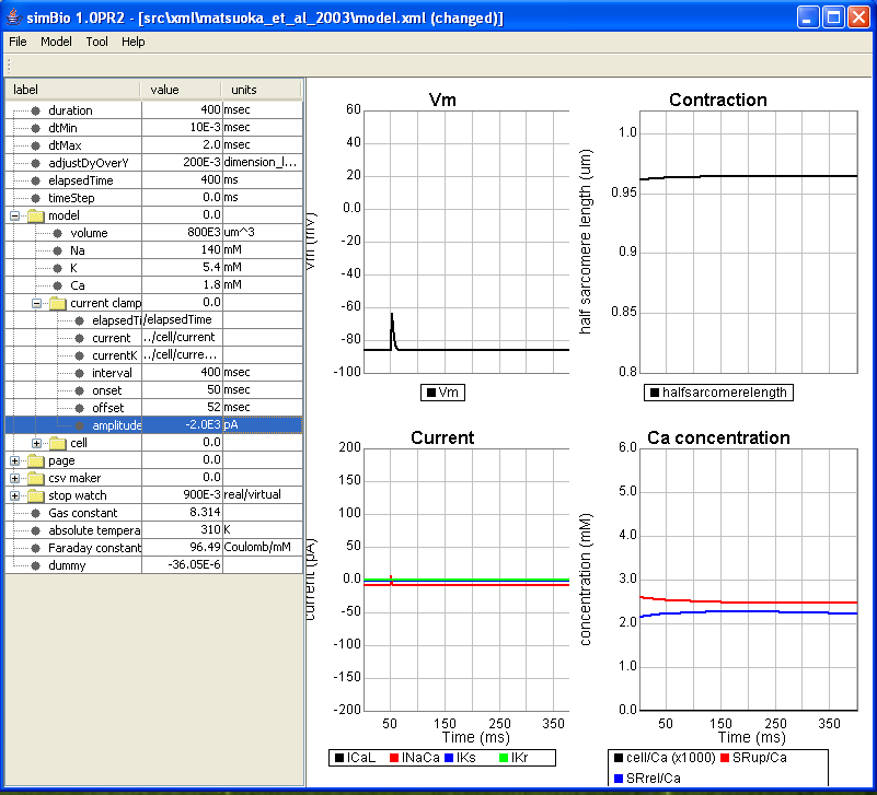
In model/current clamp/amplitude, a -4,000 pA stimulus every 400 ms (interval), from 50 ms (onset) to 52 ms (offset) is given. Here, for example when you click on the column displayed as "-4.0E3" (exponents are displayed with 3 digits) and change it to -2000 then press the Enter key, you can change the size of the stimulus to -2,000 pA.

When you click on [Start] in this state, just a small upturn is observed in 50 ms, and an action potential is not generated.

Moreover, you can change the graph display format and check the threshold at which an action potential is generated.

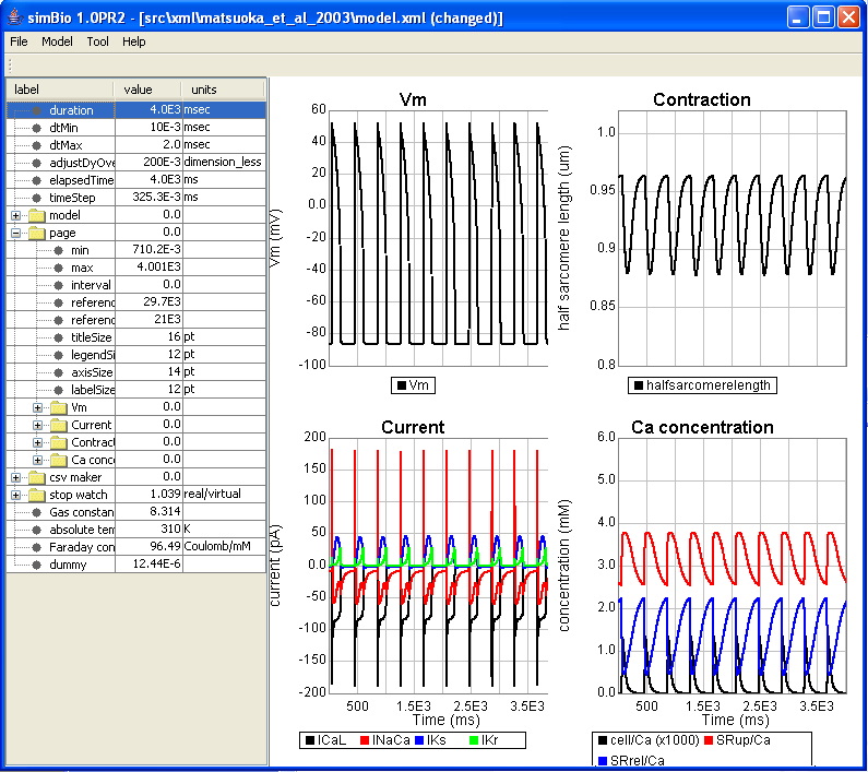
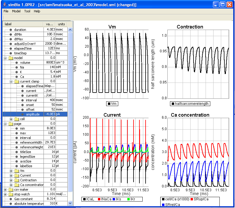
First select [Reload] from the [File] menu, and read in the initial state of src/xml/matsuoka_et_al_2003/model.xml. To change the value of the page/max parameter, click on the column in which 400 is displayed, input 4000 and press the Enter key. When you change the calculation time which is set in the duration parameter at the top to 4000 and click on [Start], you can observe that the action potential is generated 10 times in a row.

If model/current clamp/interval which is set to 400 is changed to 800, then the stimulus interval becomes longer. If it's changed to 200 then the interval becomes shorter, and the contractions and relaxations are not in time. With onset and offset timing, the stimulus current is on at 50 ms, and off at 52 ms in a stimulus cycle.

Here when you change the amplitude to -2400 and click on [Start], the phenomenon, which is called all or none, can be observed as is shown in the figure below. If the stimulus exceeds the threshold then an action potential is generated, and if it doesn't exceed the threshold, then no action potential is generated.

Next, if you return the amplitude to -4000 and click on [Start], then the phenomenon called positive staircase can be observed that the contractions gradually become a large.

In simBio, mathematical models are expressed through a network of functional element (Reactor) and parameter (Node).

A functional element (Reactor), means individual functions that can be biologically distinguished, and can be expressed with various parameters and formulas. Then combining multiple functional elements can made more complicated function elements. A parameter (Node) can be referred to and from various functional elements.

You can check the functional elements and parameters which comprise the matsuoka_et_al_2003 model by opening the model in the parameter tree table. In the model, extracellular fluid volume (volume) and ion concentrations (Na, K, Ca) are written as parameters, and stimulus electrodes (current clamp) and cell (cell) are written as function elements.

Next, when you open a cell, you can see that it consists of parameters (volume, membrane capacitance, Vm, Na, K, Ca, CaTotal, ATP) and functional elements (ATP production system, Ca binding protein, muscle contraction model, Negroni & Lascano model (1996), 18 kinds of cell membrane currents, sarcoplasmic reticulum, 4 kinds of currents on the sarcoplasmic reticulum).

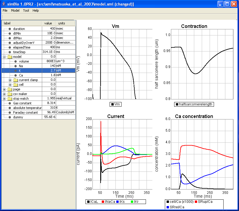
By changing the numeric values which are set here, various conditions can be set. For example, let's try changing the extracellular medium. The extracellular potassium concentration is set at model/K. If you change 5.4 mM to 2.7, then the resting potential will be hyperpolarized to more than -100 mV like in the figure below. What will happen if we change it to 10? Please look at the change in the size of the current etc.

In the same way, you can change the extracellular Na and Ca. Also, if you try changing other parts yourself, by experimenting you can try and see if known phenomena can be reproduced. In GUI [File]->[open] menu, select src/xml/sarai_et_al_2003/model.xml, and when you click on [open], the pacemaker cell model is read in.

When you run using [Start], you can see spontaneous cyclic action potentials.

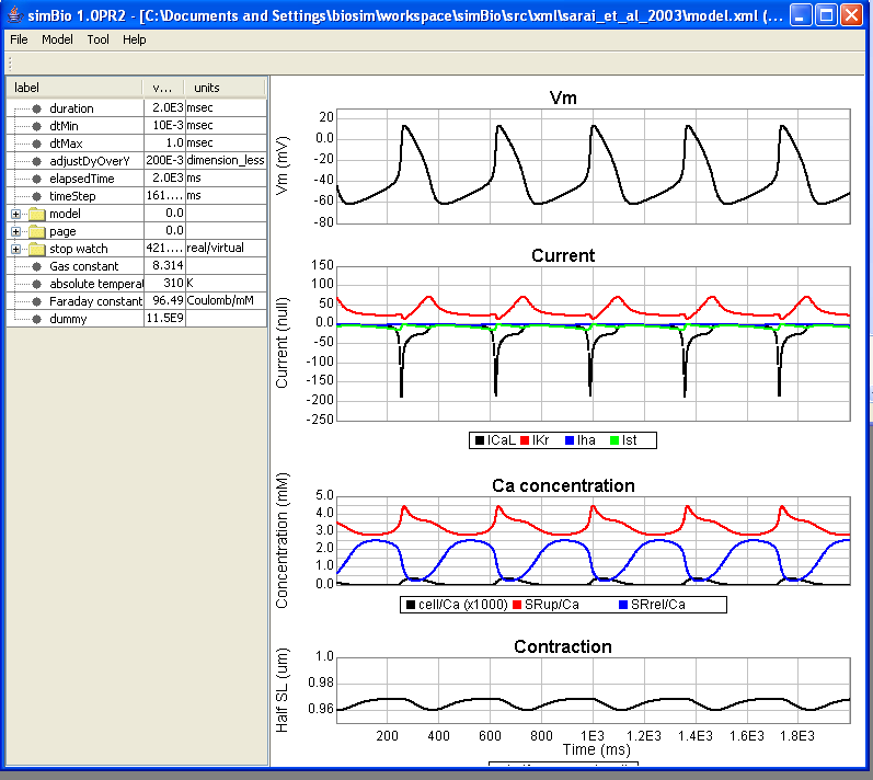
Let's change model/K which has the extracellular potassium concentration, and look at pacemaker cell activity.